Cartesium reference
Expressions and relations#
| Form | Syntax |
|---|---|
| explicit curve | sin(x) or y = sin(x) |
| implicit curve | x^2 + 3*y^2 = 1.5 |
| filled relation | x^2 + y^2 <= 16 |
| chained relation | -x^2 <= y <= x^2 |
| point | (3, 4) |
| 3D vector arrow | vector([1, 2, 3]) |
| ordered open path | polyline(xs, ys) |
| filled closed polygon | polygon(xs, ys) |
| parametric curve | (cos(t), sin(t)) {0 <= t <= 2*pi} |
| polar curve | r = 5*cos(7*theta) |
Operators are +, -, *, /, ^, =, <, <=, >, and >=.
Parentheses group expressions. Numeric juxtaposition such as 2x is
multiplication; write * between names or before a grouped expression.
Constants are pi, tau (equal to 2*pi), and e.
(x^2 + y^2)^2 = x^2 - y^2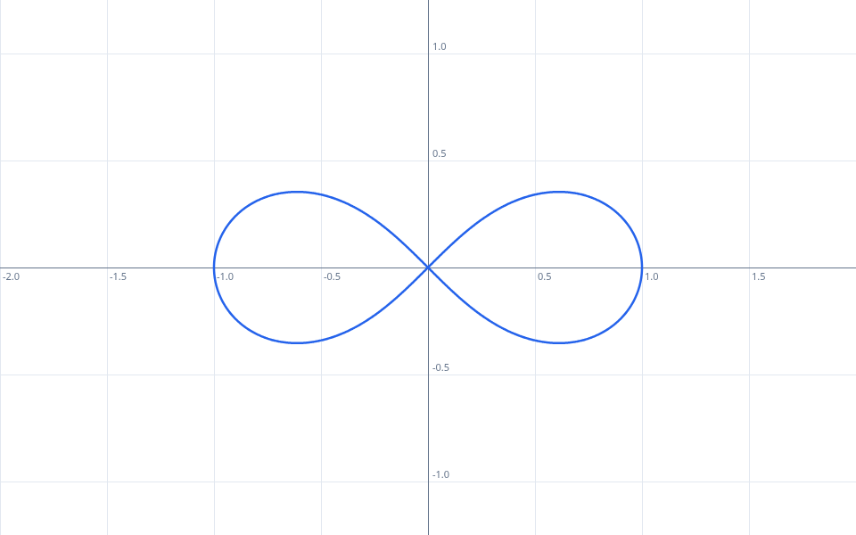
r = 5*cos(7*theta)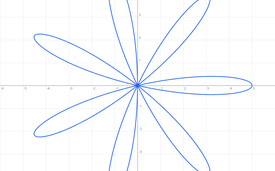
Restrictions and piecewise#
Append a condition in braces to restrict a plot:
y = sin(x) {-2*pi <= x <= 2*pi}
(cos(t), sin(t)) {0 <= t <= 2*pi}
A piecewise expression tests branches from left to right. The unlabelled final value is the fallback:
y = {x < -1: -x-1, x <= 1: x^2, x-1}Strict inequality boundaries are dashed; non-strict boundaries are solid.
y <= sin(a x)
(2*cos(t), 4*sin(t)) {0 + a <= t <= pi + a}
x^2 + y^2 >= 12
a = 1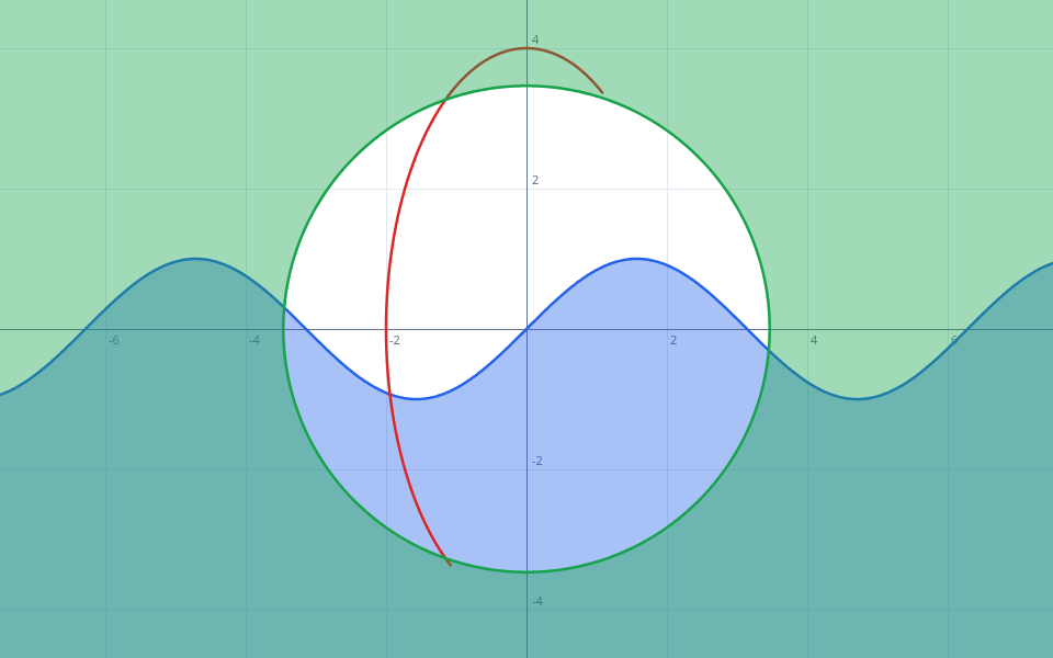
Variables and functions#
| Form | Syntax |
|---|---|
| scalar definition | a = 2 |
| function definition | f(u) = a*sin(u) |
| function call | f(x) |
| subscripted name | x_i = 3 |
| explicit named multiplication | v_i * (x - x_i) |
Definitions do not draw geometry. A numeric scalar receives slider controls; its minimum, maximum, and step are document settings. Definitions are resolved as dependencies rather than executed top to bottom.
a = 2
b = 3
f(u) = a*sin(b*u)
y = f(x)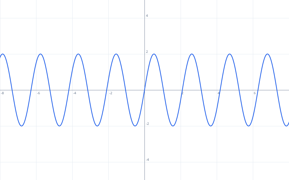
Points, polylines, and polygons#
A pair of equal-length sequences plots a point collection:
n = 1:5
(n, n^2)
Point collections do not connect their entries. Use polyline(xs, ys) to
connect equal-length coordinate sequences in order, or polygon(xs, ys) to
close the final edge and fill the enclosed path:
xs = [0, 3, 4, 2]
ys = [0, 4, 2, -1]
polygon(xs, ys)
polyline requires at least two points and polygon requires at least three.
Both preserve sequence order and duplicate vertices. Polygon orientation is
therefore retained even though clockwise and counterclockwise fills generally
look the same. Arrowheads and directed-path presentation are separate features
and are not implied by either operation.
In the 3D calculator, vector(v) draws an arrow from the origin to a finite
length-3 sequence v. An anchored form adds a tail point and a displacement: vector([4, 5, 6], [1, 2, 3]) ends at [5, 7, 9]. A zero displacement remains
valid and is shown as a point marker. An N×3 matrix draws one arrow per row, and
a single row broadcasts when paired with a matrix:
V = [1 0 0; 0 1 0; 0 0 1]
vector([0, 0, 0], V)
Anchored vectors can also be sampled over one to three finite parameter domains:
vector([x, y, 0], [y, -x, 0]) {-5 <= x <= 5} {-5 <= y <= 5}The 3D calculator samples nine points per declared axis, skips undefined samples, and keeps zero vectors as point markers. Vector collections and fields are fixed whole-scene resources; adaptive density, streamlines, and configurable arrowhead styling are not yet supported.
3D surfaces and solids#
The 3D calculator also supports implicit equalities, single-comparison solid inequalities, and explicit height surfaces:
| Form | Syntax |
|---|---|
| implicit surface | x^2 + y^2 + z^2 = 25 |
| solid inequality | x^2 + y^2 + z^2 <= 25 |
| explicit height surface | z = sin(x) * cos(y) |
A 3D inequality must contain exactly one <, <=, >, or >= comparison.
The accepted side is sampled as a signed field, and its boundary is rendered as
an opaque, double-sided surface. Strict and non-strict comparisons therefore
share the same geometric boundary, and a closed solid intentionally looks like
the corresponding hollow surface from outside. Chained or brace-restricted
inequalities, Boolean constraints, automatic plot-boundary caps, and true
volume rendering are not currently supported.
px = [-4, -1, 3, 4, 0]
py = [1, 4, 3, -1, -3]
polygon(px, py)
lx = [-4, -2, 0, 2, 4]
ly = [-3, -1, -2, 1, 0]
polyline(lx, ly)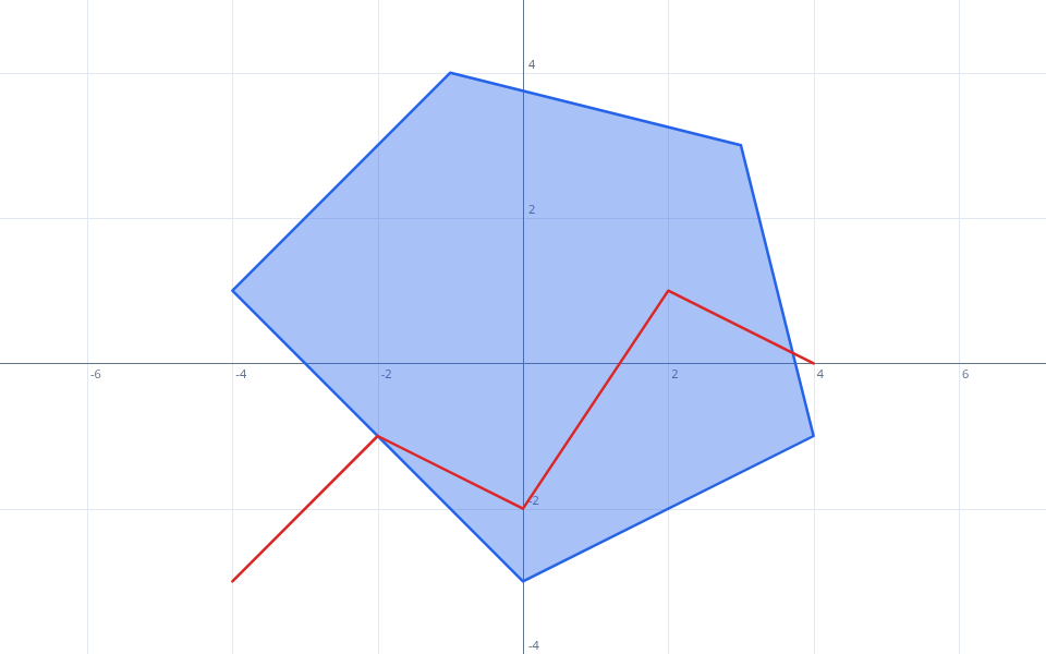
Derivatives#
| Form | Syntax |
|---|---|
| derivative operator | diff(x^3 + sin(x), x) |
| differential notation | d/dx(x^3 + sin(x)) |
| function derivative | f'(x) |
| higher derivative | f''(x) or diff(diff(f(x), x), x) |
Derivatives support arithmetic, powers, smooth elementary functions, and
compositions of user-defined functions. This includes the trigonometric,
inverse-trigonometric, reciprocal-trigonometric, hyperbolic, exponential,
logarithmic, square-root, absolute-value, and constant-degree nthroot functions listed below. atan2 and both forms of log also differentiate
structurally.
Expressions are differentiated when the expression model is built, then
evaluated through the ordinary compiled numeric path. Prime notation
differentiates the function before applying its argument, so f'(x^2) means
the value of f' at x^2, not the derivative of f(x^2). Scalar piecewise
expressions differentiate each branch while leaving variable-dependent
switching boundaries undefined. floor, ceil, round, sign, mod,
sequence extrema, reductions, and linear-algebra functions report an
unsupported-derivative diagnostic rather than claiming a derivative across
their discontinuities or non-scalar operations.
Definite integrals#
Use integral(expression, variable, lower, upper) to evaluate a finite definite
integral. For example, y = integral(sin(t), t, 0, x) plots the accumulated
area from zero to x. The integration variable is local to the integrand;
bounds may use graph variables, sliders, constants, and user-defined functions.
Reversing the bounds reverses the sign.
Definite integrals use bounded adaptive numerical quadrature. If the bounds are not finite, the integrand produces a non-finite sampled value, or the requested accuracy cannot be reached within the work limit, the result is undefined. Improper integrals and symbolic antiderivatives are not currently supported.
f(t) = sin(t)
y = f(x)
y = integral(f(t), t, 0, x)
y = 1 - cos(x)Regression#
Use ~ to fit undefined scalar parameters in a model to finite sequence data:
xs = [1, 2, 3, 4]
ys = [3.1, 4.9, 7.2, 8.8]
ys ~ m*xs + b
f(u) = m*u + b
y = f(x)
Here xs and ys are the data, while the undefined scalars m and b are
fitted by least squares. Successful regression rows display their parameters
and root-mean-square error. Fitted parameters are document-level definitions,
so later variables, functions, and plots can reuse them. An existing assignment,
such as b = 0, fixes that value instead of fitting it.
Models linear in every fitted parameter use a direct deterministic solver. This
includes polynomial models such as ys ~ a*xs^2 + b*xs + c: the powers of the
data do not make the parameters nonlinear.
Genuinely nonlinear models use bounded nonlinear least squares. For example:
ys ~ a*exp(b*xs) + c
ys ~ a*xs^b
ys ~ l/(1 + exp(-k*(xs - x0)))
ys ~ a*sin(b*xs + c) + d
Nonlinear fitting is iterative and can have multiple local solutions, particularly for sinusoidal models. The solver tries a deterministic set of starting points and reports the best finite solution it finds; equivalent parameterizations can therefore display different parameter values for the same curve. A nonlinear relation may fit at most 8 parameters and 20,000 data rows. All regression data must be nonempty and equally sized, and the supplied data must independently determine every fitted parameter.
Sequences and ranges#
| Form | Syntax | Result |
|---|---|---|
| literal | [1, 3, 5] | ordered values |
| unit range | 1:5 | [1, 2, 3, 4, 5] |
| stepped range | 1:2:9 | [1, 3, 5, 7, 9] |
| comprehension | [n^2 for n in 1:5] | [1, 4, 9, 16, 25] |
| one-based index | values[2] | second value |
| slice | values[2:4] | second through fourth values |
| indexed selection | values[[1, 3]] | first and third values |
Scalar arithmetic broadcasts over sequences. Equal-length sequences support
elementwise + and -; .* is elementwise multiplication.
k = 400
radius = [0.7*sqrt(n) for n in 0:k]
angle = [n*pi*(3-sqrt(5)) for n in 0:k]
(radius.*cos(angle), radius.*sin(angle))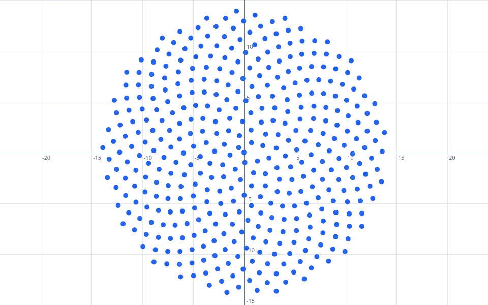
Vectors and matrices#
One-dimensional sequences are vectors. In matrix literals, spaces separate columns and semicolons separate rows. Indexing is one-based.
| Operation | Syntax |
|---|---|
| matrix literal | A = [1 2; 3 4] |
| vector literal | v = [5, 6] |
| matrix element | A[2, 1] |
| matrix-vector product | A * v |
| matrix-matrix product | A * B |
| scalar product | 2 * A |
| inner product | dot(v, w) |
| elementwise product | v .* w |
| Euclidean norm | norm(v) |
| transpose | transpose(A) |
A * [x, y] <= b is the conjunction of the component inequalities and draws
their feasible region.
A = [-1 0; 0 -1; 2 1; 1 3]
b = [0, 0, 8, 9]
A * [x, y] <= b
c = [3, 2]
z = 8
y = (z-c[1]*x)/c[2]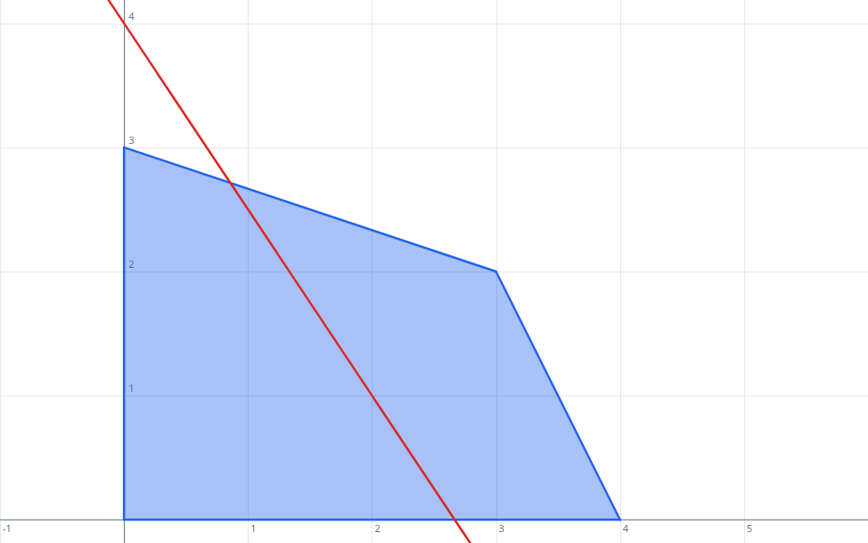
A = [-1 0; 1 -2; -2 1]
b = [0, 0, 0]
A * [x, y] <= b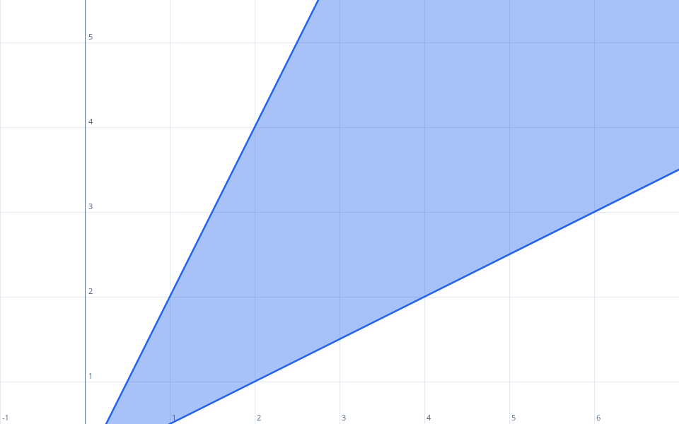
Built-in functions#
| Kind | Functions |
|---|---|
| trigonometric | sin, cos, tan, sec, csc, cot |
| inverse trigonometric | asin, acos, atan, atan2(y, x) |
| hyperbolic | sinh, cosh, tanh |
| exponential and logarithmic | exp, ln, log(x), log(x, base) |
| roots and magnitude | sqrt, nthroot(x, n), abs |
| rounding, sign, and remainder | floor, ceil, round, sign, mod(x, m) |
| extrema | min, max |
| sequence | length, sum, product, mean, unique |
| linear algebra | dot, norm, transpose |
log(x) is base 10; use ln(x) for the natural logarithm or log(x, base) for another base. Logarithms require a positive argument and a positive base
other than one. atan2(y, x) uses the signs of both coordinates to select the
angle’s quadrant. nthroot(x, n) requires nonzero n and supports negative x when n is an odd integer. For nonzero m, mod(x, m) returns the
Euclidean remainder from zero up to, but not including, abs(m).
min and max accept one or more arguments. atan2, nthroot, mod, and dot take two; log takes one or two; the remaining built-ins take one.
Scalar functions broadcast over sequences, pairing equal-length sequence
arguments element by element. Unary scalar functions also map over matrices.
The built-in constants are pi, tau, and e.
Styling and animation#
Visible curves expose color, width, and opacity. Inequalities also expose fill opacity. Point collections instead expose color, marker opacity, pixel radius, and marker shape: disc, annulus, cross, square, diamond, or triangle.
Variables and function definitions have no plot style and do not consume the automatic color sequence. Numeric variables expose slider bounds, step, playback speed, direction, and repeat behavior.
Graph settings control axes, grids, bounds, equal axis scale, and appearance. Drag the panel edge to resize the expression panel; double-click the edge to reset it. Drag to pan; use the wheel or a pinch gesture to zoom.
Saving, sharing, and embedding#
| Action | Result |
|---|---|
| Save | updates the current browser draft, or the signed-in private Space document |
| Save As | new browser draft while signed out; new private Space document when Spaces is enabled and signed in |
| My graphs | manage browser drafts, private Space documents, and signed-in publications |
| Share | compressed, self-contained snapshot in #doc= |
| Publish | immutable listed or unlisted public publicationV2 record in the user’s AT Protocol PDS |
| Export PNG | image of the current viewport |
Snapshot links open as unsaved copies and require no server-side anonymous record. Embedded graphs show a still preview until activated. Only one embed on a page owns a live renderer; Expand shows its read-only expression list and Edit opens an editable copy.
When Spaces is disabled or the user is signed out, browser drafts are labeled Browser only and are not synced. With Spaces enabled, a signed-in Save As creates a mutable document in the account’s personal Space; public listed and unlisted publications remain separate immutable records.